Where a pilgrim's map comes from

Dham Navigator has one stubborn promise: it works with the radio off. A pilgrim should be able to stand anywhere in the dham — no signal, no guide, a dead SIM — and still see where they are, what happened there, and the footpath to the next place. Keeping that promise means one thing above all: everything is already on the phone before they ever arrive. The streets, the hills, the buildings, the temples, the stories, the walking routes — all of it ships inside the app.

So the natural question, and the subject of this whole piece, is: where does every one of those pieces come from, what format is it once it’s sitting on the device, and how do we make it? The data has two very different parents.

Some of it is borrowed from the world’s open maps and generated by a machine — OpenStreetMap, the European Space Agency’s elevation model, building datasets from Overture and Google. We don’t draw the streets of Vṛndāvana by hand; we extract them. This data is reproducible: delete it, run a script, get it back.

The rest is written by us, and this is the soul of the guide: which places matter, what happened at each one, the photograph that helps you recognise a temple from the road, the traditional parikrama. No algorithm produces that.

Everything below ships per region — Vṛndāvana, Māyāpur and Barsana so far — into a single folder of files the app reads straight off local storage. There is no database and no live server behind the map.

Everything at a glance

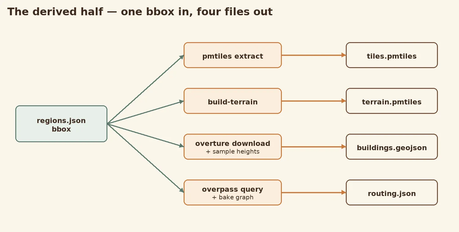
One config file, regions.json, holds nothing but each region’s bounding box and zoom range — the entire derived pipeline keys off it:

{
  "vrindavan": { "bbox": [77.66, 27.548, 77.73, 27.605], "maxzoom": 16,
                 "geofabrikZone": "asia/india/northern-zone", "terrain": true },
  "barsana":   { "bbox": [77.355, 27.63, 77.405, 27.67],  "maxzoom": 16,
                 "geofabrikZone": "asia/india/northern-zone", "terrain": true }
}

From that, each region ends up with a handful of files. Here is the whole cast, what it is, and where it comes from:

File	Format	What it is	Origin
tiles.pmtiles	PMTiles, vector	the base map	derived — OSM
terrain.pmtiles	PMTiles, raster-DEM	the hills	derived — Copernicus DEM
buildings.geojson	GeoJSON polygons	building footprints + height	derived — Overture + Google
routing.json	JSON graph	the walking network	derived — OSM via Overpass
locations.geojson	GeoJSON points	curated places	hand-authored
locations/<id>.json	JSON	a place’s photos	hand-authored
locations/<id>.<lang>.md	Markdown	a place’s story	hand-authored
routes.json	JSON	preset parikramas	hand-authored
models.geojson + .glb	GeoJSON + glTF	3-D landmark models	hand-authored

The rest of this article walks each one — first the four we generate, then the ones we write.

The base map

The streets, rivers, ghats, parks and labels come from OpenStreetMap, the same open map that powers a good part of the internet. We take a daily global build from Protomaps, cut out just the few square kilometres around each dham, and store it as a single PMTiles file — one tidy archive of vector tiles, around a megabyte per region:

pmtiles extract https://build.protomaps.com/<date>.pmtiles \
  tiles.pmtiles --bbox=77.355,27.63,77.405,27.67 --maxzoom=15

Drawn flat, those vector layers are the canvas everything else sits on — the greens of Maangarh hill, the kuṇḍas in blue, the lanes, and every building:

That single-file part matters more than it sounds. Because it’s one range-readable archive, MapLibre — the renderer — pulls just the slice it needs for what’s on screen, straight from the phone’s own storage, no network. That’s the trick that lets a whole town’s map live in a megabyte and open instantly in airplane mode. The licence is OpenStreetMap’s ODbL; the app credits it in the About screen.

The walking network

When you tap two points and the app draws a path between them, it isn’t guessing — it’s walking a graph we built from OpenStreetMap’s footpaths. A script asks the Overpass API for walkable ways only (footways, paths, steps, residential lanes, tracks — motorways left out, because a pilgrim walks the small roads), then bakes them into a compact graph: every junction becomes a node, every stretch of road an edge weighted by its real length in metres.

The ask to Overpass is just a highway filter over the region’s bounding box — keep the walkable classes, drop the rest:

way["highway"~"^(footway|path|pedestrian|steps|living_street|residential|
  service|track|unclassified|tertiary|secondary|primary|cycleway|bridleway)$"]
  (s, w, n, e);

That graph, drawn straight from the file we ship, is the actual road network of Barsana — the village core, with the lanes radiating out into the fields:

On disk it is deliberately tiny — just coordinates and connections, no geometry flourish:

{ "bbox": [77.355, 27.63, 77.405, 27.67],
  "nodes": [[77.2755, 27.6554], [77.2761, 27.6551], …],
  "edges": [[0, 1, 64.0], [1, 2, 85.6], [2, 3, 118.4], …] }

A node’s identity is just its index in the array; an edge is [from, to, metres], where the weight is the great-circle distance between its two endpoints — the haversine of their longitudes and latitudes:

$$d = 2R\arcsin\sqrt{\sin^2\tfrac{\Delta\varphi}{2} + \cos\varphi_1\cos\varphi_2\sin^2\tfrac{\Delta\lambda}{2}}$$

with $R$ the Earth’s radius, 6,371 km. Barsana’s network is 1,231 nodes and 1,252 edges and weighs about 46 KB; Vṛndāvana, a far denser town, runs ten times that. At load the app turns this into an adjacency list and runs A* over it — and because the graph is labelled by connected component, route endpoints snap onto the same reachable island of road (the fix for Māyāpur, whose OSM coverage is still patchy).

The hills — a height map hidden in a picture

Barsana is built on hills. Śrīmatī Rādhārāṇī’s village rises out of the plain, and a flat map flattens that story away. So for Barsana we ship terrain — the relief you can see and tilt — and the elevation behind it is the most quietly clever piece of data in the whole app.

It comes from Copernicus DEM, the European Space Agency’s free global elevation model: for every 30 metres of ground, a measured height above sea level, served as Cloud-Optimized GeoTIFFs we read directly over HTTPS — no full download. The catch is that “height” isn’t naturally a picture, and our renderer speaks pictures. The solution is the Terrarium encoding: each elevation is packed into the red, green and blue of a single pixel.

$$\text{elevation} = R \times 256 + G + \frac{B}{256} - 32768$$

Stored, that looks like a meaningless wash of green. Decoded with the formula above, the hills come back:

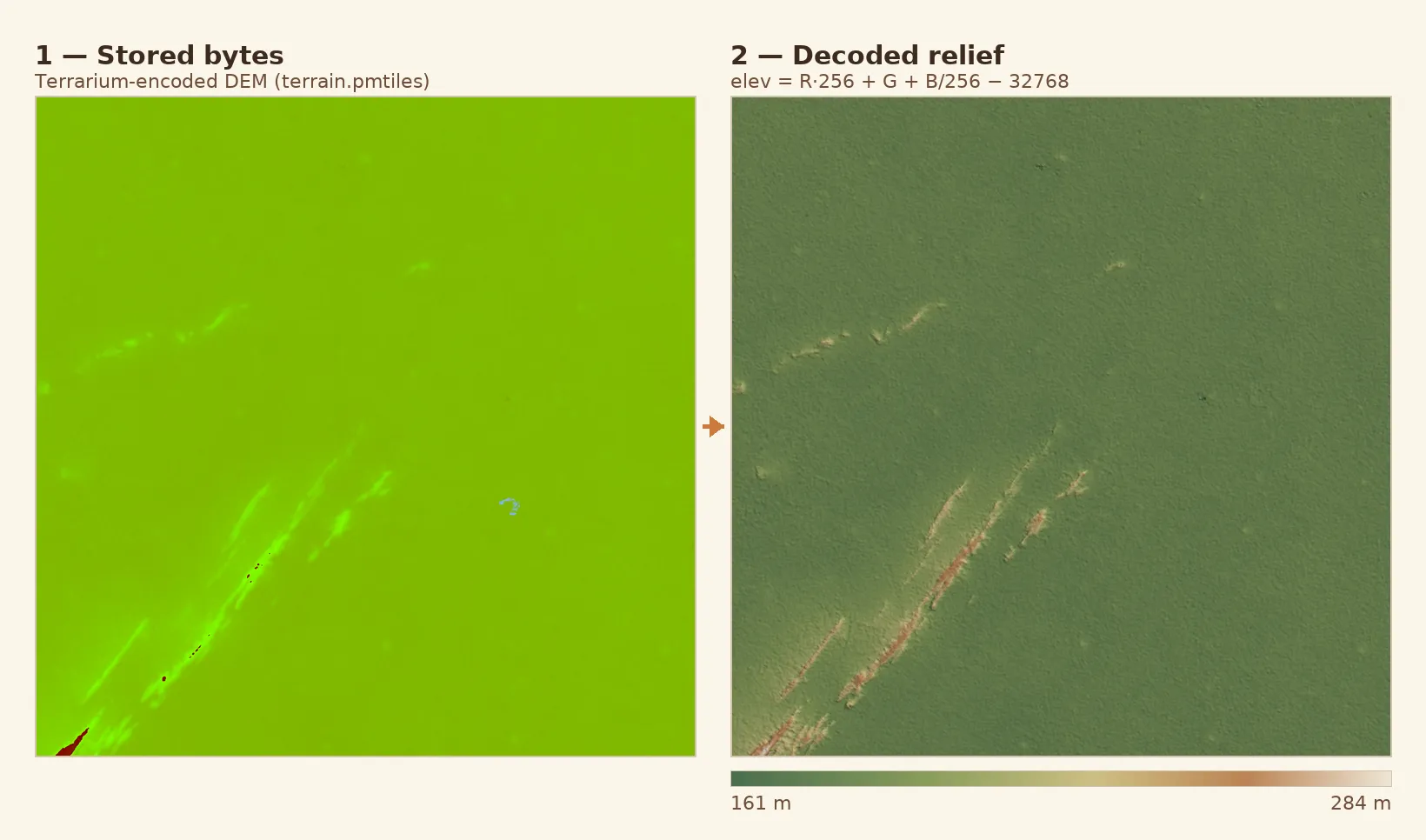
On the left is exactly the kind of data sitting in terrain.pmtiles — just coloured bytes. On the right is the same pixels after the phone runs the formula: Barsana’s ridges emerge, rising from about 160 metres on the plain to 285 at the peaks. The app reverses the encoding in real time to lift the surface into a 3-D mesh and cast hillshade across it. Vṛndāvana and Māyāpur, on the flat Yamunā and Gaṅgā plains, skip terrain entirely — there’s no relief worth the battery.

Hillshade — lighting the slopes

A height map is just numbers; relief is something the eye reads. So from the same DEM we compute a hillshade. For each pixel we look at its neighbours to work out which way the ground slopes and how steeply — its aspect and gradient — and then light it from a fixed sun angle. Ground facing the sun turns bright; ground facing away falls into shadow, and all at once the flat grid of numbers looks like hills.

Concretely, from the 3×3 patch of elevations around each cell (Horn’s method) we take the gradient, which gives the slope $S$ and the direction the ground faces, the aspect $A$. With the sun at zenith angle $Z$ and azimuth $A_\odot$, the brightness of the cell is a single dot product:

$$\text{shade} = \cos Z \cos S + \sin Z \sin S \cos(A_\odot - A)$$

In code it is barely more — exactly what generated the picture below:

// gradient from the 3×3 neighbourhood (a,b,c / d,·,f / g,h,i), z-exaggerated
const dzdx = ((c + 2*f + i) - (a + 2*d + g)) / (8 * cellMetres) * zFactor
const dzdy = ((g + 2*h + i) - (a + 2*b + c)) / (8 * cellMetres) * zFactor
const slope  = Math.atan(Math.hypot(dzdx, dzdy))
const aspect = Math.atan2(dzdy, -dzdx)
let shade = Math.cos(zenith) * Math.cos(slope)
          + Math.sin(zenith) * Math.sin(slope) * Math.cos(azimuth - aspect)
shade = Math.max(0, shade)            // 0 = shadow, 1 = full sun

The map renderer does the same thing live, on the GPU, straight from the Terrarium tiles; we tint the shadows a warm brown and the highlights cream so the relief sits inside the palette instead of fighting it. Run it over Barsana and the village’s namesake hill, and the ridges of the parikramā rise out of the plain:

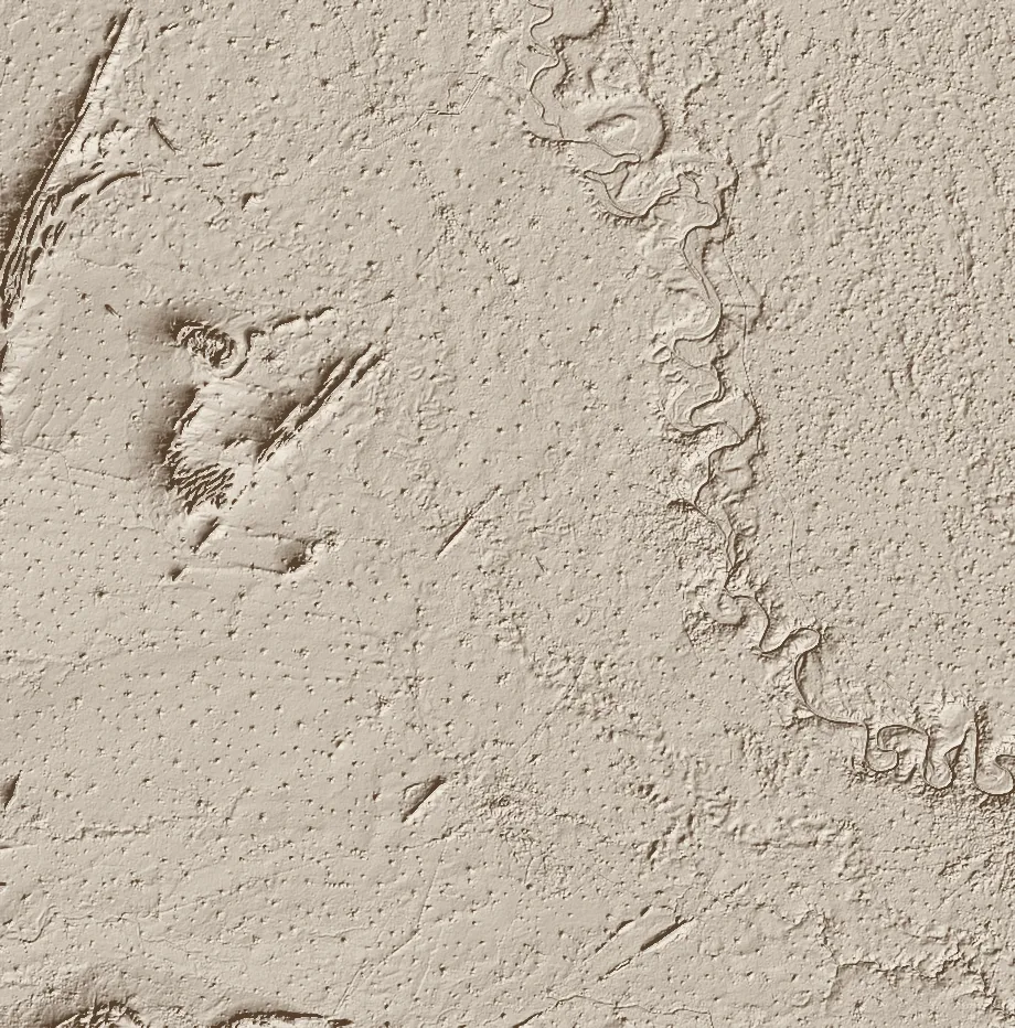
Generated for this article straight from the Copernicus GLO-30 DEM — per-pixel slope and aspect, lit from the north-west. The faint speckle is the surface model catching rooftops and trees.

And the same shading, live and pannable, computed in your browser from the real terrain.pmtiles:

The buildings

The shapes standing up on the map are real building footprints from Overture Maps, an open dataset backed by Meta, Microsoft, Amazon and others. One command pulls every footprint inside the bounding box:

overturemaps download --bbox=77.355,27.63,77.405,27.67 \
  -t building -f geojson -o buildings.geojson

We strip each one to bare geometry and store the lot as plain GeoJSON — a list of polygons. Barsana has 7,738 of them. Coloured by height, the village draws itself:

Each feature is as plain as it looks — a polygon and one number:

{ "type": "Feature",
  "properties": { "height": 8.1 },
  "geometry": { "type": "Polygon",
    "coordinates": [[[77.356037, 27.630412], [77.356112, 27.630492], …]] } }

But where does that height come from? Overture gives us the shape of each building, not how tall it is. That’s a second dataset, and a small algorithm.

How a building gets its height

The heights come from Google Open Buildings, which publishes a raster — a grid of pixels, roughly one every four metres — where each pixel’s value is the estimated building height at that spot on the ground. To turn that into a single height for one footprint, we lay the polygon over the raster, look at every pixel it covers, and take the tallest one — so a temple’s śikhara wins over the courtyard beside it:

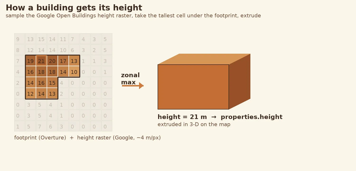
It is a zonal maximum — walk every cell under the footprint on a 2-metre grid and keep the tallest, so a tower beats the courtyard a centroid might land in:

let best = 0                                   // metres
for (const [x, y] of cellsUnder(footprint, 2)) // 2 m sampling grid
  best = Math.max(best, sampleHeight(x, y) ?? 0)
feature.properties.height = Math.round(best * 10) / 10

That number becomes properties.height, and the map extrudes the flat footprint into a 3-D block of exactly that height. Footprints the dataset is unsure about — the very large complexes, like a big temple — come back as zero and get filled in by hand. The heights are licensed CC-BY-4.0, so the app credits Google Open Buildings alongside Overture and OSM.

The part we write by hand

Everything above gives you a beautiful, accurate map. It does not give you a guidebook. That part we author ourselves, place by place.

The places that matter

locations.geojson is our curated index — temples, ghāts, kuṇḍas and samādhis, each a single point with a stable id, a kind, and its name in English and Russian. These are the dots you tap. Drawn over the road network, the 13 places of Barsana look like this:

{ "type": "Feature",
  "properties": { "id": "maan-mandir", "kind": "temple",
                  "name:en": "Shri Maan Mandir", "name:ru": "Шри Ман Мандир" },
  "geometry": { "type": "Point", "coordinates": [77.3655119, 27.6434345] } }

These coordinates are ours, not scraped: a few are checked against OpenStreetMap, but most come from field-GPS readings and the old books, entered one at a time. The file stays deliberately light — just enough to draw a dot and power search — so the heavy content loads only when you open a place.

The story and photographs of each place

A place’s rich content lives in two sibling files keyed by the same id, loaded lazily the moment its card opens. Take Shri Maan Mandir, the temple on Maangarh hill that we labelled on the map above. Its story is just Markdown — locations/maan-mandir.en.md:

A temple on Maangarh hill marking the place where Srimati Radharani showed her
loving sulk (maan) toward Krishna. It overlooks Barsana and is a centre of daily
seva and kirtan.

One file per language, so a visit becomes darśana and not just sightseeing; raw Markdown means translators edit the prose directly and changes read cleanly in a diff. Its photos sit beside it in locations/maan-mandir.json, each listing its variants — a full-size original and a thumbnail — with dimensions:

{ "id": "maan-mandir",
  "photos": [{
    "description": { "en": "Maan Mandir on Maangarh hill", "ru": "Ман Мандир на холме Мангарх" },
    "variants": [
      { "type": "original",  "path": "photos/maan-mandir/01.original.jpg",  "width": 1600, "height": 1067 },
      { "type": "thumbnail", "path": "photos/maan-mandir/01.thumbnail.jpg", "width": 500,  "height": 333 }
    ] }] }

The photos themselves are the one thing that doesn’t ship inside the app — they’d make it huge. The manifest stores only a relative path, never a full address; the actual JPEGs stream from our own image server the first time you open a place, then cache on the phone for good. Storing a path and not a URL means we can move the whole photo library to a new host by changing a single line, with no data to migrate.

The routes

routes.json holds the traditional walks — the Vṛndāvana parikrama and the like — as an ordered list of stops. Each stop is either a reference to a curated place or a raw shaping point that steers the path, and the whole thing runs through the same footpath router as a route you draw yourself.

Landmark models

For the most important temples we go one step further than an extruded box: a hand-made 3-D model, a glTF .glb file, placed on the map by a tiny models.geojson that says where it stands and how big it is. This is just beginning — one model so far, the Madana-mohana temple in Vṛndāvana — but it’s the same idea as everything else here: a small file of data, authored once, rendered offline.

How it all comes together

Two halves, one map. The derived half is machine-made from open data; the authored half is hand-made by us; together they become a single region’s map, every layer stacked in one place:

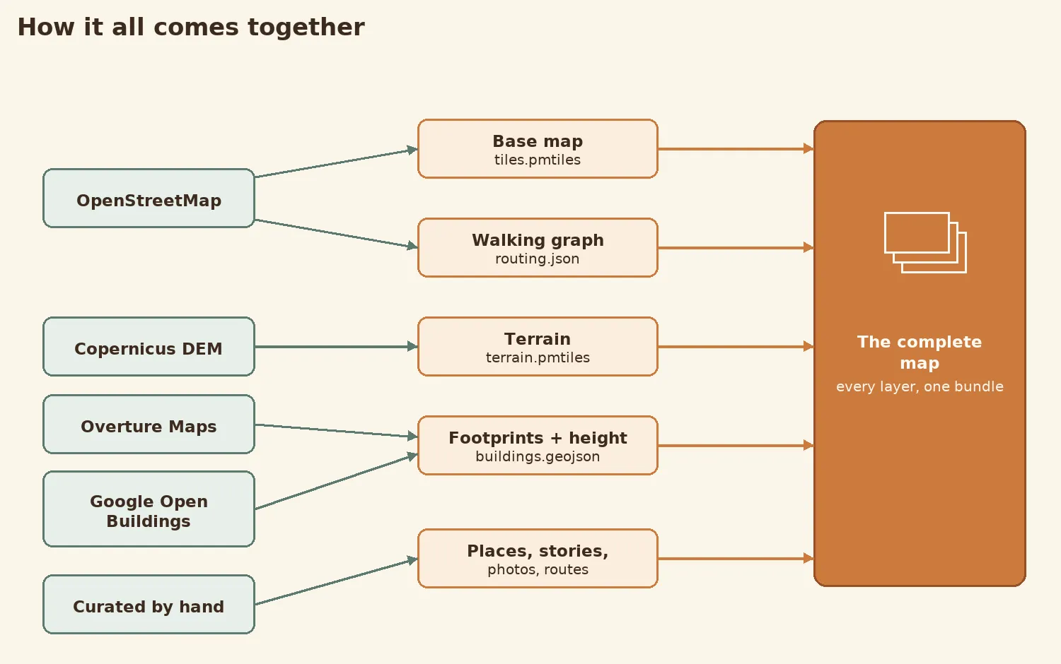
And the derived half, in more detail — every script reads the one regions.json bounding box and writes one file:

That’s the whole pipeline: the open world’s maps for the ground beneath your feet, and our own hands for everything that makes the ground holy — folded together into something that fits in a pocket and never needs a signal.

The result

Everything in this article stacks into a single frame, drawn by the very same MapLibre engine the app uses. Bottom to top, it registers the layers in this order:

flowchart TB
  M["Terrain mesh (from the DEM)"] --> A["Land, water and green fills"]
  A --> H["Hillshade"]
  H --> R["Roads — white lines"]
  R --> B["Buildings — 3D extrusion"]

The Copernicus hills lifted into a mesh and shaded by hillshade; the building footprints standing up at their Google-measured heights; the OpenStreetMap lanes drawn in white; the kuṇḍas picked out in water — every layer from this article, in one place.

And here it is, live — Barsana, composited in 3-D right here in the page. Drag to orbit, scroll to zoom, tilt to feel the hills:

No tile server, no signal — just the handful of files we built, rendered in your browser exactly as they are rendered in the palm of a hand, deep in the dham.